Manipulating Data with dplyr
Overview
dplyr is an R package for working with structured data both in and outside of R. dplyr makes data manipulation for R users easy, consistent, and performant. With dplyr as an interface to manipulating Spark DataFrames, you can:
- Select, filter, and aggregate data
- Use window functions (e.g. for sampling)
- Perform joins on DataFrames
- Collect data from Spark into R
Statements in dplyr can be chained together using pipes defined by the magrittr R package. dplyr also supports non-standard evalution of its arguments. For more information on dplyr, see the introduction, a guide for connecting to databases, and a variety of vignettes.
Reading Data
You can read data into Spark DataFrames using the following functions:
| Function | Description |
|---|---|
spark_read_csv |
Reads a CSV file and provides a data source compatible with dplyr |
spark_read_json |
Reads a JSON file and provides a data source compatible with dplyr |
spark_read_parquet |
Reads a parquet file and provides a data source compatible with dplyr |
Regardless of the format of your data, Spark supports reading data from a variety of different data sources. These include data stored on HDFS (hdfs:// protocol), Amazon S3 (s3n:// protocol), or local files available to the Spark worker nodes (file:// protocol)
Each of these functions returns a reference to a Spark DataFrame which can be used as a dplyr table (tbl).
Flights Data
This guide will demonstrate some of the basic data manipulation verbs of dplyr by using data from the nycflights13 R package. This package contains data for all 336,776 flights departing New York City in 2013. It also includes useful metadata on airlines, airports, weather, and planes. The data comes from the US Bureau of Transportation Statistics, and is documented in ?nycflights13
Connect to the cluster and copy the flights data using the copy_to function. Caveat: The flight data in nycflights13 is convenient for dplyr demonstrations because it is small, but in practice large data should rarely be copied directly from R objects.
library(sparklyr)
library(dplyr)
library(nycflights13)
library(ggplot2)

sc <- spark_connect(master="local")
flights <- copy_to(sc, flights, "flights")
airlines <- copy_to(sc, airlines, "airlines")
src_tbls(sc)
## [1] "airlines" "flights"dplyr Verbs
Verbs are dplyr commands for manipulating data. When connected to a Spark DataFrame, dplyr translates the commands into Spark SQL statements. Remote data sources use exactly the same five verbs as local data sources. Here are the five verbs with their corresponding SQL commands:
select~SELECTfilter~WHEREarrange~ORDERsummarise~aggregators: sum, min, sd, etc.mutate~operators: +, *, log, etc.
select(flights, year:day, arr_delay, dep_delay)## # Source: lazy query [?? x 5]
## # Database: spark_connection
## year month day arr_delay dep_delay
## <int> <int> <int> <dbl> <dbl>
## 1 2013 1 1 11 2
## 2 2013 1 1 20 4
## 3 2013 1 1 33 2
## 4 2013 1 1 -18 -1
## 5 2013 1 1 -25 -6
## 6 2013 1 1 12 -4
## 7 2013 1 1 19 -5
## 8 2013 1 1 -14 -3
## 9 2013 1 1 -8 -3
## 10 2013 1 1 8 -2
## # ... with more rowsfilter(flights, dep_delay > 1000)## # Source: lazy query [?? x 19]
## # Database: spark_connection
## year month day dep_time sched_dep_time dep_delay arr_time
## <int> <int> <int> <int> <int> <dbl> <int>
## 1 2013 1 9 641 900 1301 1242
## 2 2013 1 10 1121 1635 1126 1239
## 3 2013 6 15 1432 1935 1137 1607
## 4 2013 7 22 845 1600 1005 1044
## 5 2013 9 20 1139 1845 1014 1457
## # ... with 12 more variables: sched_arr_time <int>, arr_delay <dbl>,
## # carrier <chr>, flight <int>, tailnum <chr>, origin <chr>, dest <chr>,
## # air_time <dbl>, distance <dbl>, hour <dbl>, minute <dbl>,
## # time_hour <dbl>arrange(flights, desc(dep_delay))## # Source: table<flights> [?? x 19]
## # Database: spark_connection
## # Ordered by: desc(dep_delay)
## year month day dep_time sched_dep_time dep_delay arr_time
## <int> <int> <int> <int> <int> <dbl> <int>
## 1 2013 1 9 641 900 1301 1242
## 2 2013 6 15 1432 1935 1137 1607
## 3 2013 1 10 1121 1635 1126 1239
## 4 2013 9 20 1139 1845 1014 1457
## 5 2013 7 22 845 1600 1005 1044
## 6 2013 4 10 1100 1900 960 1342
## 7 2013 3 17 2321 810 911 135
## 8 2013 6 27 959 1900 899 1236
## 9 2013 7 22 2257 759 898 121
## 10 2013 12 5 756 1700 896 1058
## # ... with more rows, and 12 more variables: sched_arr_time <int>,
## # arr_delay <dbl>, carrier <chr>, flight <int>, tailnum <chr>,
## # origin <chr>, dest <chr>, air_time <dbl>, distance <dbl>, hour <dbl>,
## # minute <dbl>, time_hour <dbl>summarise(flights, mean_dep_delay = mean(dep_delay))## # Source: lazy query [?? x 1]
## # Database: spark_connection
## mean_dep_delay
## <dbl>
## 1 12.63907mutate(flights, speed = distance / air_time * 60)## # Source: lazy query [?? x 20]
## # Database: spark_connection
## year month day dep_time sched_dep_time dep_delay arr_time
## <int> <int> <int> <int> <int> <dbl> <int>
## 1 2013 1 1 517 515 2 830
## 2 2013 1 1 533 529 4 850
## 3 2013 1 1 542 540 2 923
## 4 2013 1 1 544 545 -1 1004
## 5 2013 1 1 554 600 -6 812
## 6 2013 1 1 554 558 -4 740
## 7 2013 1 1 555 600 -5 913
## 8 2013 1 1 557 600 -3 709
## 9 2013 1 1 557 600 -3 838
## 10 2013 1 1 558 600 -2 753
## # ... with more rows, and 13 more variables: sched_arr_time <int>,
## # arr_delay <dbl>, carrier <chr>, flight <int>, tailnum <chr>,
## # origin <chr>, dest <chr>, air_time <dbl>, distance <dbl>, hour <dbl>,
## # minute <dbl>, time_hour <dbl>, speed <dbl>Laziness
When working with databases, dplyr tries to be as lazy as possible:
It never pulls data into R unless you explicitly ask for it.
It delays doing any work until the last possible moment: it collects together everything you want to do and then sends it to the database in one step.
For example, take the following code:
c1 <- filter(flights, day == 17, month == 5, carrier %in% c('UA', 'WN', 'AA', 'DL'))
c2 <- select(c1, year, month, day, carrier, dep_delay, air_time, distance)
c3 <- arrange(c2, year, month, day, carrier)
c4 <- mutate(c3, air_time_hours = air_time / 60)
This sequence of operations never actually touches the database. It’s not until you ask for the data (e.g. by printing c4) that dplyr requests the results from the database.
c4## # Source: lazy query [?? x 8]
## # Database: spark_connection
## # Ordered by: year, month, day, carrier
## year month day carrier dep_delay air_time distance air_time_hours
## <int> <int> <int> <chr> <dbl> <dbl> <dbl> <dbl>
## 1 2013 5 17 AA -2 294 2248 4.900000
## 2 2013 5 17 AA -1 146 1096 2.433333
## 3 2013 5 17 AA -2 185 1372 3.083333
## 4 2013 5 17 AA -9 186 1389 3.100000
## 5 2013 5 17 AA 2 147 1096 2.450000
## 6 2013 5 17 AA -4 114 733 1.900000
## 7 2013 5 17 AA -7 117 733 1.950000
## 8 2013 5 17 AA -7 142 1089 2.366667
## 9 2013 5 17 AA -6 148 1089 2.466667
## 10 2013 5 17 AA -7 137 944 2.283333
## # ... with more rowsPiping
You can use magrittr pipes to write cleaner syntax. Using the same example from above, you can write a much cleaner version like this:
c4 <- flights %>%
  filter(month == 5, day == 17, carrier %in% c('UA', 'WN', 'AA', 'DL')) %>%
  select(carrier, dep_delay, air_time, distance) %>%
  arrange(carrier) %>%
  mutate(air_time_hours = air_time / 60)
Grouping
The group_by function corresponds to the GROUP BY statement in SQL.
c4 %>%
  group_by(carrier) %>%
  summarize(count = n(), mean_dep_delay = mean(dep_delay))
## # Source: lazy query [?? x 3]
## # Database: spark_connection
## carrier count mean_dep_delay
## <chr> <dbl> <dbl>
## 1 AA 94 1.468085
## 2 DL 136 6.235294
## 3 UA 172 9.633721
## 4 WN 34 7.970588Collecting to R
You can copy data from Spark into R’s memory by using collect().
carrierhours <- collect(c4)collect() executes the Spark query and returns the results to R for further analysis and visualization.
# Test the significance of pairwise differences and plot the results
with(carrierhours, pairwise.t.test(air_time, carrier))
##
## Pairwise comparisons using t tests with pooled SD
##
## data: air_time and carrier
##
## AA DL UA
## DL 0.25057 - -
## UA 0.07957 0.00044 -
## WN 0.07957 0.23488 0.00041
##
## P value adjustment method: holmggplot(carrierhours, aes(carrier, air_time_hours)) + geom_boxplot()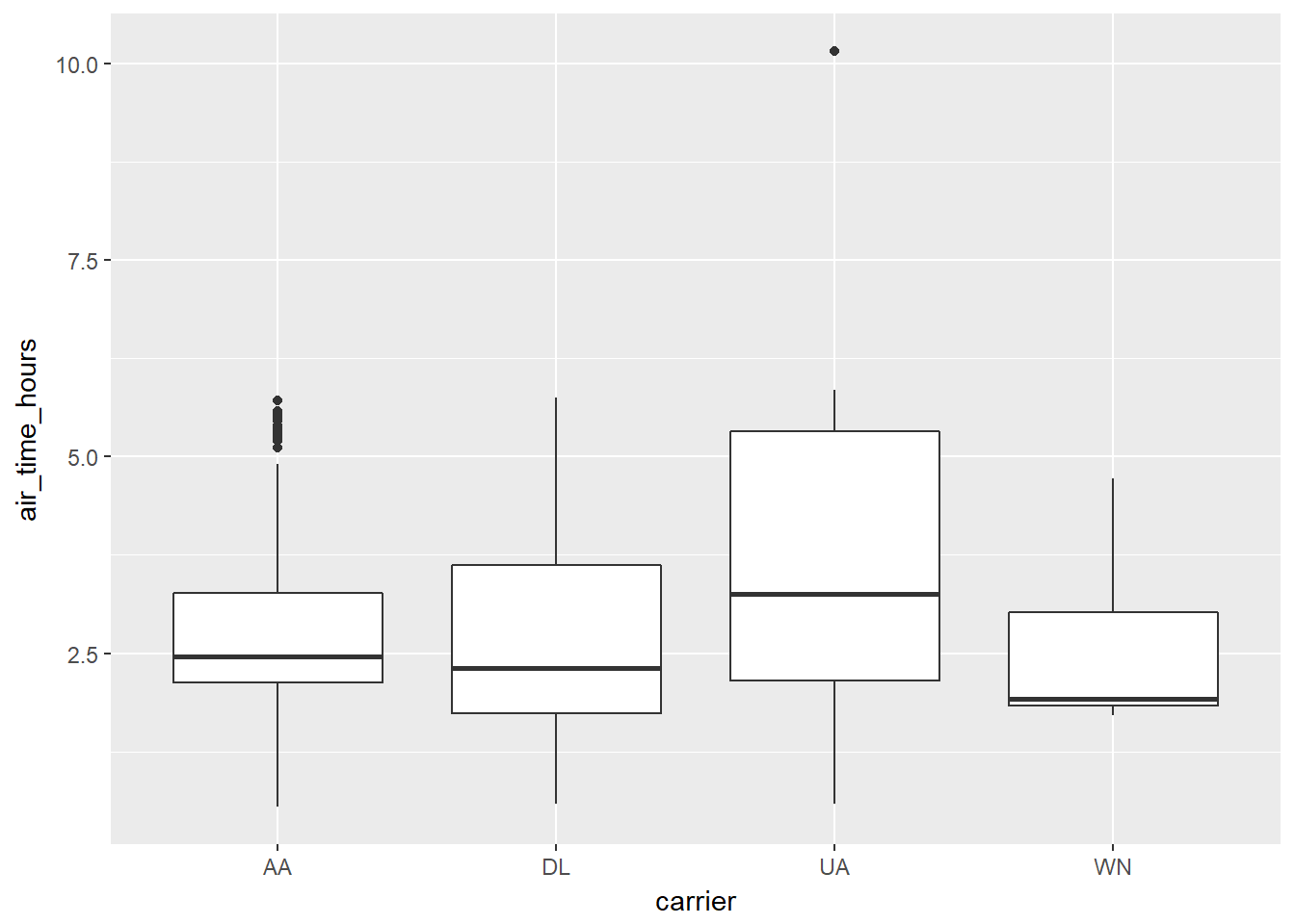
If you want to execute a query and store the results in a temporary table, use compute()
compute(c4, 'carrierhours')## # Source: lazy query [?? x 5]
## # Database: spark_connection
## # Ordered by: carrier
## carrier dep_delay air_time distance air_time_hours
## <chr> <dbl> <dbl> <dbl> <dbl>
## 1 AA -7 142 1089 2.366667
## 2 AA -9 186 1389 3.100000
## 3 AA -6 143 1096 2.383333
## 4 AA -4 114 733 1.900000
## 5 AA -2 146 1085 2.433333
## 6 AA -7 119 733 1.983333
## 7 AA -3 193 1598 3.216667
## 8 AA -7 137 944 2.283333
## 9 AA -1 195 1389 3.250000
## 10 AA -2 294 2248 4.900000
## # ... with more rowssrc_tbls(sc)## [1] "airlines" "carrierhours" "flights"SQL Translation
It’s relatively straightforward to translate R code to SQL (or indeed to any programming language) when doing simple mathematical operations of the form you normally use when filtering, mutating and summarizing. dplyr knows how to convert the following R functions to Spark SQL:
# Basic math operators
+, -, *, /, %%, ^

# Math functions
abs, acos, asin, asinh, atan, atan2, ceiling, cos, cosh, exp, floor, log, log10, round, sign, sin, sinh, sqrt, tan, tanh

# Logical comparisons
<, <=, !=, >=, >, ==, %in%

# Boolean operations
&, &&, |, ||, !

# Character functions
paste, tolower, toupper, nchar

# Casting
as.double, as.integer, as.logical, as.character, as.date

# Basic aggregations
mean, sum, min, max, sd, var, cor, cov, n
Window Functions
dplyr supports Spark SQL window functions. Window functions are used in conjunction with mutate and filter to solve a wide range of problems. You can compare the dplyr syntax to the query it has generated by using dbplyr::sql_render().
# Find the most and least delayed flight each day
bestworst <- flights %>%
  group_by(year, month, day) %>%
  select(dep_delay) %>%
  filter(dep_delay == min(dep_delay) || dep_delay == max(dep_delay))
dbplyr::sql_render(bestworst)
## <SQL> SELECT `year`, `month`, `day`, `dep_delay`
## FROM (SELECT `year`, `month`, `day`, `dep_delay`, min(`dep_delay`) OVER (PARTITION BY `year`, `month`, `day`) AS `zzz5`, max(`dep_delay`) OVER (PARTITION BY `year`, `month`, `day`) AS `zzz6`
## FROM (SELECT `year` AS `year`, `month` AS `month`, `day` AS `day`, `dep_delay` AS `dep_delay`
## FROM `flights`) `hgpnrplbmd`) `xmxtutmkid`
## WHERE (`dep_delay` = `zzz5` OR `dep_delay` = `zzz6`)
bestworst
## # Source:   lazy query [?? x 4]
## # Database: spark_connection
## # Groups:   year, month, day
##     year month   day dep_delay
##    <int> <int> <int>     <dbl>
##  1  2013     1     1       853
##  2  2013     1     1       -15
##  3  2013     1     1       -15
##  4  2013     1     9      1301
##  5  2013     1     9       -17
##  6  2013     1    24       -15
##  7  2013     1    24       329
##  8  2013     1    29       -27
##  9  2013     1    29       235
## 10  2013     2     1       -15
## # ... with more rows
# Rank each flight within a daily
ranked <- flights %>%
group_by(year, month, day) %>%
select(dep_delay) %>%
mutate(rank = rank(desc(dep_delay)))
dbplyr::sql_render(ranked)## <SQL> SELECT `year`, `month`, `day`, `dep_delay`, rank() OVER (PARTITION BY `year`, `month`, `day` ORDER BY `dep_delay` DESC) AS `rank`
## FROM (SELECT `year` AS `year`, `month` AS `month`, `day` AS `day`, `dep_delay` AS `dep_delay`
## FROM `flights`) `bhmotnqley`ranked## # Source: lazy query [?? x 5]
## # Database: spark_connection
## # Groups: year, month, day
## year month day dep_delay rank
## <int> <int> <int> <dbl> <int>
## 1 2013 1 1 853 1
## 2 2013 1 1 379 2
## 3 2013 1 1 290 3
## 4 2013 1 1 285 4
## 5 2013 1 1 260 5
## 6 2013 1 1 255 6
## 7 2013 1 1 216 7
## 8 2013 1 1 192 8
## 9 2013 1 1 157 9
## 10 2013 1 1 155 10
## # ... with more rowsPeforming Joins
It’s rare that a data analysis involves only a single table of data. In practice, you’ll normally have many tables that contribute to an analysis, and you need flexible tools to combine them. In dplyr, there are three families of verbs that work with two tables at a time:
Mutating joins, which add new variables to one table from matching rows in another.
Filtering joins, which filter observations from one table based on whether or not they match an observation in the other table.
Set operations, which combine the observations in the data sets as if they were set elements.
All two-table verbs work similarly. The first two arguments are x and y, and provide the tables to combine. The output is always a new table with the same type as x.
The following statements are equivalent:
flights %>% left_join(airlines)## Joining, by = "carrier"## # Source: lazy query [?? x 20]
## # Database: spark_connection
## year month day dep_time sched_dep_time dep_delay arr_time
## <int> <int> <int> <int> <int> <dbl> <int>
## 1 2013 1 1 517 515 2 830
## 2 2013 1 1 533 529 4 850
## 3 2013 1 1 542 540 2 923
## 4 2013 1 1 544 545 -1 1004
## 5 2013 1 1 554 600 -6 812
## 6 2013 1 1 554 558 -4 740
## 7 2013 1 1 555 600 -5 913
## 8 2013 1 1 557 600 -3 709
## 9 2013 1 1 557 600 -3 838
## 10 2013 1 1 558 600 -2 753
## # ... with more rows, and 13 more variables: sched_arr_time <int>,
## # arr_delay <dbl>, carrier <chr>, flight <int>, tailnum <chr>,
## # origin <chr>, dest <chr>, air_time <dbl>, distance <dbl>, hour <dbl>,
## # minute <dbl>, time_hour <dbl>, name <chr>flights %>% left_join(airlines, by = "carrier")## # Source: lazy query [?? x 20]
## # Database: spark_connection
## year month day dep_time sched_dep_time dep_delay arr_time
## <int> <int> <int> <int> <int> <dbl> <int>
## 1 2013 1 1 517 515 2 830
## 2 2013 1 1 533 529 4 850
## 3 2013 1 1 542 540 2 923
## 4 2013 1 1 544 545 -1 1004
## 5 2013 1 1 554 600 -6 812
## 6 2013 1 1 554 558 -4 740
## 7 2013 1 1 555 600 -5 913
## 8 2013 1 1 557 600 -3 709
## 9 2013 1 1 557 600 -3 838
## 10 2013 1 1 558 600 -2 753
## # ... with more rows, and 13 more variables: sched_arr_time <int>,
## # arr_delay <dbl>, carrier <chr>, flight <int>, tailnum <chr>,
## # origin <chr>, dest <chr>, air_time <dbl>, distance <dbl>, hour <dbl>,
## # minute <dbl>, time_hour <dbl>, name <chr>flights %>% left_join(airlines, by = c("carrier", "carrier"))## # Source: lazy query [?? x 20]
## # Database: spark_connection
## year month day dep_time sched_dep_time dep_delay arr_time
## <int> <int> <int> <int> <int> <dbl> <int>
## 1 2013 1 1 517 515 2 830
## 2 2013 1 1 533 529 4 850
## 3 2013 1 1 542 540 2 923
## 4 2013 1 1 544 545 -1 1004
## 5 2013 1 1 554 600 -6 812
## 6 2013 1 1 554 558 -4 740
## 7 2013 1 1 555 600 -5 913
## 8 2013 1 1 557 600 -3 709
## 9 2013 1 1 557 600 -3 838
## 10 2013 1 1 558 600 -2 753
## # ... with more rows, and 13 more variables: sched_arr_time <int>,
## # arr_delay <dbl>, carrier <chr>, flight <int>, tailnum <chr>,
## # origin <chr>, dest <chr>, air_time <dbl>, distance <dbl>, hour <dbl>,
## # minute <dbl>, time_hour <dbl>, name <chr>Sampling
You can use sample_n() and sample_frac() to take a random sample of rows: use sample_n() for a fixed number and sample_frac() for a fixed fraction.
sample_n(flights, 10)## # Source: lazy query [?? x 19]
## # Database: spark_connection
## year month day dep_time sched_dep_time dep_delay arr_time
## <int> <int> <int> <int> <int> <dbl> <int>
## 1 2013 1 1 517 515 2 830
## 2 2013 1 1 533 529 4 850
## 3 2013 1 1 542 540 2 923
## 4 2013 1 1 544 545 -1 1004
## 5 2013 1 1 554 600 -6 812
## 6 2013 1 1 554 558 -4 740
## 7 2013 1 1 555 600 -5 913
## 8 2013 1 1 557 600 -3 709
## 9 2013 1 1 557 600 -3 838
## 10 2013 1 1 558 600 -2 753
## # ... with more rows, and 12 more variables: sched_arr_time <int>,
## # arr_delay <dbl>, carrier <chr>, flight <int>, tailnum <chr>,
## # origin <chr>, dest <chr>, air_time <dbl>, distance <dbl>, hour <dbl>,
## # minute <dbl>, time_hour <dbl>sample_frac(flights, 0.01)## # Source: lazy query [?? x 19]
## # Database: spark_connection
## year month day dep_time sched_dep_time dep_delay arr_time
## <int> <int> <int> <int> <int> <dbl> <int>
## 1 2013 1 1 711 715 -4 1151
## 2 2013 1 1 752 759 -7 955
## 3 2013 1 1 857 900 -3 1124
## 4 2013 1 1 936 945 -9 1257
## 5 2013 1 1 1109 1115 -6 1402
## 6 2013 1 1 1245 1249 -4 1722
## 7 2013 1 1 1400 1400 0 1634
## 8 2013 1 1 1657 1650 7 1921
## 9 2013 1 1 1859 1900 -1 2012
## 10 2013 1 2 558 600 -2 838
## # ... with more rows, and 12 more variables: sched_arr_time <int>,
## # arr_delay <dbl>, carrier <chr>, flight <int>, tailnum <chr>,
## # origin <chr>, dest <chr>, air_time <dbl>, distance <dbl>, hour <dbl>,
## # minute <dbl>, time_hour <dbl>Writing Data
It is often useful to save the results of your analysis or the tables that you have generated on your Spark cluster into persistent storage. The best option in many scenarios is to write the table out to a Parquet file using the spark_write_parquet function. For example:
spark_write_parquet(tbl, "hdfs://hdfs.company.org:9000/hdfs-path/data")This will write the Spark DataFrame referenced by the tbl R variable to the given HDFS path. You can use the spark_read_parquet function to read the same table back into a subsequent Spark session:
tbl <- spark_read_parquet(sc, "data", "hdfs://hdfs.company.org:9000/hdfs-path/data")You can also write data as CSV or JSON using the spark_write_csv and spark_write_json functions.
Hive Functions
Many of Hive’s built-in functions (UDF) and built-in aggregate functions (UDAF) can be called inside dplyr’s mutate and summarize. The Languange Reference UDF page provides the list of available functions.
The following example uses the datediff and current_date Hive UDFs to figure the difference between the flight_date and the current system date:
flights %>%
  mutate(flight_date = paste(year,month,day,sep="-"),
         days_since = datediff(current_date(), flight_date)) %>%
  group_by(flight_date,days_since) %>%
  tally() %>%
  arrange(-days_since)
## # Source: lazy query [?? x 3]
## # Database: spark_connection
## # Groups: flight_date
## # Ordered by: -days_since
## flight_date days_since n
## <chr> <int> <dbl>
## 1 2013-1-1 1777 842
## 2 2013-1-2 1776 943
## 3 2013-1-3 1775 914
## 4 2013-1-4 1774 915
## 5 2013-1-5 1773 720
## 6 2013-1-6 1772 832
## 7 2013-1-7 1771 933
## 8 2013-1-8 1770 899
## 9 2013-1-9 1769 902
## 10 2013-1-10 1768 932
## # ... with more rows